
INSIGHTS Research
By Leo Carlos-Sandberg, 05/10/2021
Hi, I’m Leo, an AI Researcher at Arabesque AI working in research and development. Specifically, I focus on our input data, analysing it, understanding its structure and processing it. I have a background in finance, computer science, and physics and have seen how all three disciplines deal with complex systems. This piece will give an overview of complex systems, their importance, and some associated challenges. I’ve written this overview to illustrate the difficulty of understanding financial markets and the need for highly sophisticated approaches.
Complex systems
Whether or not you realise it, your life has been impacted by complex systems. These systems are everywhere and lead to much of the complexity associated with decision making in the natural world. A complex system is a system composed of interacting components. Some well-known complex systems are the human brain (interacting neurons), social group structures (interacting people), gases (interacting particles), and financial markets (interacting market participants). Often, multiple different complex systems can be derived from a single system. Take, for example, financial markets; complex systems may be composed of traded assets (for stock price analysis), banks (for bankruptcy risk analysis), and non-market values with traded assets (for an investigation of the impact of ESG data on stock price).
Emergent behaviour
The construction of a complex system is often simple, merely composed of interacting components, furthermore in many cases these components and/or interactions are themselves simple in nature and well understood. However, even simple components with simple interactions can, at a large scale, exhibit a phenomenon known as emergent behaviour. Emergent behaviour can be seen as the complex behaviour of a system that is not immediately obvious from its individual interactions. A perfect example of emergent behaviour is illustrated in Conway’s Game of Life, a 2D grid where each square (cell) may be either black or white (alive or dead) based on the following rules:
1. Any live cell with two or three live neighbours survives.
2. Any dead cell with three live neighbours becomes a live cell.
3. All other live cells die in the next generation. Similarly, all other dead cells stay dead.
This game is given an initial configuration and then repeatedly iterated (with each iteration being a new generation) based on the above rules. This setup is relatively simple but can lead to the occurrence of some impressive emergent behaviour, as shown below. In fact, this game is Turing complete1, and from these simple rules, people have even been able to make the Game of Life within the Game of Life!

This emergent behaviour becomes important for real-world systems, though it can be benign, it may also be beneficial or harmful. An example of harmful emergent behaviour is ‘hot potato trading’ between high-frequency market markers. This behaviour causes a market maker to buy assets and then rapidly sell them to another market maker who repeats the process (similar to passing a hot potato between a group of people). This artificially increases the trading volume of the asset heavily affecting the market price. Some hypothesise that this behaviour was a significant contributor to the 2010 flash crash. More broadly, emergent behaviour can also be seen in financial markets in the form of regimes defining high-level market behaviours, such as bubbles.
Due to the potentially significant impact of these emergent behaviours, those participating in the markets should have methods incorporating these complexities to make well-informed decisions.
A popular approach to investigating emergent behaviour is through simulation, which is often done in two stages. First, a model of the system is created by building pieces of code to act as each component in the system, and allowing these components to exchange information. These types of models are referred to as agent-based models. These models can be given initial conditions and run, allowing for emergent behaviour to occur naturally in a system that is amenable to analysis (with its interactions and behaviours tracked). Second, due to the randomness associated with running these models (or the lack of knowledge on the initial conditions) to gather an idea of the system these models will be run many times (under different conditions) with the results aggregated. This approach is known as a Monte Carlo method.
Relation discovery
So far, we have been discussing systems under the assumption that we know how the components interact; however, in reality this is rarely the case. Interactions are often unknown and challenging to discover, with the naive perturbation methods (impacting one component to see how others react) being either impossible or immoral (for very good reason, it is illegal to intentionally crash a market to see the reaction). Because of this, practitioners typically rely on statistical inference methods (methods that use data or results from the system to infer structure and knowledge of the system) to determine the relationship between components. Inference methods are particularly useful when considering data that is often not directly associated with the stock price, and hence the interactions are harder to infer, such as ESG data.
Statistical inference of relationships between components relies on a measurable output of each component; taking an example system composed of US technology companies, one could use the stock price of each of these companies. This naturally takes the form of a time series2 that then represents the company’s state throughout time, multiple time series of this type can then be compared to explore how the components of a system interact throughout time.
For time series data, relationship discovery often takes one of two conceptual approaches. Either the similar movement of the series, or the predictive information content of the series. Here we will discuss these by briefly describing two popular and straightforward methods, Pearson correlation, for the former, and Granger causality, for the latter. Pearson correlation measures how similar the movement of two series are, i.e. if one increases by an amount over time, does the other also increase? A strong correlation is often taken to imply that two components are linked. However, as the adage goes, correlation does not equal causation, and many things with a high correlation are obviously not linked, such as the decrease in pirates and the increase in global warming. A potentially more robust approach to relationship discovery is Granger causality. This is a measure of how much the past of one series can be used to predict the future of another series, over the predictive power of that series’ own history, e.g. if a series X and Y are identical, there would be no Granger causality, but there would be correlation. This measure has a sense of direction, where one variable “causes” another, and considers how much a series may predict itself. Both measures are quite simple, being based on linearity and bivariate systems, and many more simple and complex approaches exist.
Relationship patterns
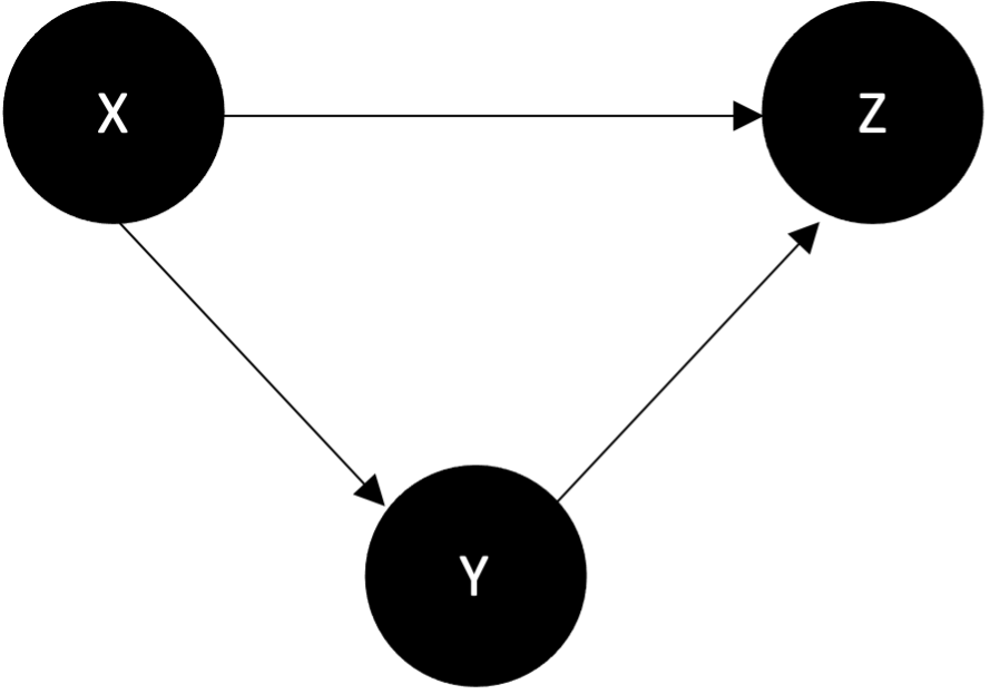
Often statistical inference of relationships is discussed in the context of two variables, e.g. given X and Y, does one cause the other. However in reality it is unlikely that the approximation that a system is composed of only two variables, will hold. This is because most real-world systems have confounding variables (which is especially relevant when considering causation), that may affect both X and Y, e.g. a confounding variable Z may cause both X and Y, which can appear as X causing Y even though that is not the case. This makes statistical inference of causation and relationships within multivariate systems significantly more complex and challenging. These confounding variables need to be considered as the systems cannot be decomposed into bivariate ones.
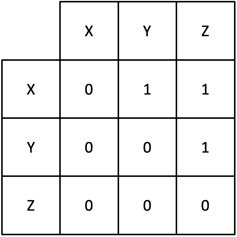
To represent the relationship information of a multivariate system matrices are often used, frequently referred to as patterns preceded by the type of relationship being shown, e.g. causality pattern. An example of how a network of causality links can be encoded as a pattern is shown below3:
Time-varying relationships
Another level of complexity with real-world systems is that these relationships are frequently dynamic, changing in strength and even existence over time. Though this dynamic behaviour likely has logical and understandable causes, these may be occurring at such a low level as to not be viewable when modelling or analysing the system; for example, the investment strategy of an individual investor might change if that investor is about to go on holiday and wants to clear their positions, however investor’s vacation calendars are rarely public knowledge. Therefore, when discussing complex systems, it is likely that the components themselves could in theory be described by another system, and that these components’ behaviour is the emergent behaviour of that system. This abstraction (turning systems into components of larger systems) through introducing some level of randomness is necessary. If we were to build a true full model of a system it would require considering the entire universe and every particle in it, which is somewhat impractical.
Though systems do not exist in isolation many outside effects may be negligible or considered as noise, which, if kept at an appropriate level can be acceptable for a given objective. This type of abstraction can be seen in measures such as temperature: while technically a measure of particle excitement, its abstraction to a Celsius temperature (a simpler measure) is more appropriate for everyday use. Another example is in finance, where modelling the logic of every single investor may not be needed, and instead their actions may be taken as overall trends and behaviours, with deviations considered as noise.
To transform statistical approaches for inference of static relationships into ones for time-varying relationships windowing is frequently employed. Windowing breaks the time series data into segments, where the aforementioned methods can be applied to each segment sequentially instead of to the whole series. This produces a new series, where each item in the series is the matrix of relationships for the system during that segment. However, this introduces its own issues with one wanting short windows to capture short term behaviour but longer windows providing more robust statistical estimation.
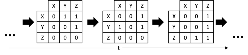
The behaviour of these changing interactions (trying to find logic and predictability within it) is another area of research, adding even more complexity to these types of systems.
Concluding remarks
In this blog, I have gone through some causes of complexity in understanding, modelling, and predicting complex systems, such as financial markets. It should now be apparent that financial markets are rife with complex, multi-level, and non-obvious behaviours and connections. The analysis of financial markets is by no means a solved problem. To gain a greater understanding of its complex and dynamic nature, advanced tools and techniques need to be developed and implemented. This type of advancement can be seen in the work done here at Arabesque AI.
Footnotes:
1: In principle a Turing complete system could be used to solve any computation problem [8].
2: A time series is a sequence of data points that occur consecutively over a time period.
3: In the network diagram circles represent components of the system and arrows the causal links between them. In the causality pattern 0 represents no causality and 1 represents a causal link.
References:
McKenzie. R. H, 2017, Emergence in the Game of Life, blogspot, viewed 1 September 2021, <https://condensedconcepts.blogspot.com/2017/09/emergence-in-game-of-life.html >
Bradbury. P, 2012, Life in life, youtube, viewed 10 September 2021, <https://www.youtube.com/watch?v=xP5-iIeKXE8>
Court. E, 2013, ‘The Instability of Market-Making Algorithms’, MEng Dissertation, UCL, London
Benesty. J, Chen. J, Hung. Y, & Cohen. I, 2009, ‘Pearson Correlation Coefficient’, Noise Reduction in Speech Processing, vol. 2, pp. 1-4
Granger. C, 1969, ‘Investigating Causal Relations by Econometric Models and Cross-Spectral Methods’, Econometrica, vol. 37, pp. 424-438
Andersen. E, 2012, True Fact: The Lack of Pirates is Causing Global Warming, Forbes, viewed 2 September 2021, < https://www.forbes.com/sites/erikaandersen/2012/03/23/true-fact-the-lack-of-pirates-is-causing-global-warming/?sh=3a6520033a67 >
Jiang. M, Gao. X, An. H, Li. H, & Sun. B, 2017, ‘Reconstructing complex network for characterizing the time-varying causality evolution behavior of multivariate time series’, Scientific Reports, https://doi.org/10.1038/s41598-017-10759-3
Sellin. E, 2017, What exactly is Turing Completeness?, evin sellin medium, viewed 3 September 2021, <http://evinsellin.medium.com/what-exactly-is-turing-completeness-a08cc36b26e2>