Symmetries, supervision and stocks: what computer vision can teach us about applying AI to finance
Date: 2021-07-26
Source: Arabesque
By Dr Tom McAuliffe – Arabesque AI
In order to find an edge in hyper-competitive markets, at Arabesque AI we utilise ideas with their roots in a wide range of research areas, including computer science, maths, and physics. In this blog post we'll consider computer vision (CV), a subfield of machine learning focused on the automated analysis of images. Artificial intelligence as a whole owes much of its success to breakthroughs in CV, and its broader relevance persists today.
During the early 2010s the video gaming industry was booming, contributing to an increased supply of affordable graphical processing units (GPUs). This brought the back-propagation algorithm back into prominence for neural network training – perfectly suited for the massively parallel capabilities of GPUs. The ImageNet challenge conceived by Li et al [1] in 2006, asks competitors to classify 14 million photographs into one of approximately 20,000 categories; by leveraging the power of GPUs, in 2012 the AlexNet [2] convolutional neural network (CNN) surpassed all competition. It achieved an error rate marginally over 15%, almost 11% better than its closest rival. This breakthrough in CV, powered by ImageNet, CNNs, and GPU-powered back-propagation was a paradigm shift for artificial intelligence.
In the pursuit of out-of-sample generalisation, classes of models have emerged that are very well suited to specific types of data. To understand why the CNN is particularly well equipped for the analysis of images, we need to take a closer look at its architecture – what is convolution?
Images are just grids of pixels. In order to generate useful (from an ML point of view) features from these pixels, one traverses a small matrix (filter) across the grid, from top left to bottom right, first performing a pixel-wise (or element-wise in matrix terms) multiplication of filter and target pixels, followed by summing the results (perform dot-products)[1]. This is schematically shown in Figure 1. Depending on the filters chosen, we can highlight specific features of the image, as shown in Figure 2 (in all figures we use 3-by-3 pixel filters). The 'Sobel' filters used in Figure 2 (b) and (c) correspond to highlighting abrupt changes in the horizontal and vertical directions respectively. The gradient (or 'Scharr') filter in (d) identifies object boundaries independent of direction. These are simple, linear examples. In a CNN, rather than specifying a-priori what the filter matrices should be, we allow the system to learn the optimal filters for the problem at hand. Rather than identifying horizontal edges, with enough complexity (neural network depth) a CNN learns to identify features as abstract as "cat ears" or "human faces". This is achieved through hierarchical combinations of simpler features (like the horizontal-edge Sobel filter) noted above, akin to the human visual system [3].
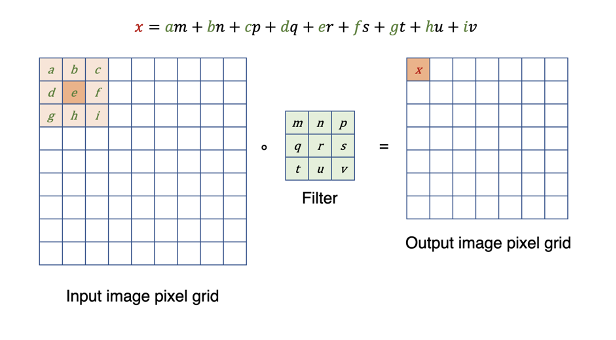
Figure 1: Operation of a convolutional filter

Figure 2: Variously filtered images
In the years since AlexNet, we have seen increasingly highly performing architectures that, under certain conditions, transfer extremely well to other domains despite having been developed for more specialised subfields. Key examples of this are the CNN for CV and the Transformer for natural language processing. The transferability ultimately stems from shared symmetries in data. Convolutional models are so successful for CV applications because they utilise inherent symmetries present in natural images. As we saw in the simple example demonstrated in Figures 1 and 2, a 2D convolutional filter scans across a 2D image[2]. This very act of scanning a filter across the image is itself exploiting the fact that by definition, images emerge as strongly local groupings at multiple nested scales. Cat-ear pixels are very likely to be adjacent to additional cat-ear pixels, lending the possibility of an appropriately tuned filter specifically for cat-ears. As humans we have evolved to consider this concept as stating-the-obvious, but the same logic does not apply, for example, to rows and columns of a spreadsheet. Independent entries (rows) can be completely unrelated to nearby entries, and there is no importance to the ordering of the columns (features). If you were to randomly shuffle the columns of an image, the meaning would be completely lost.

Figure 3: Shuffled tabular data
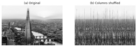
Figure 4: Shuffled image data
In Machine Learning nomenclature, this type of resistance-to-shuffling is called translational symmetry. It is a property of images but is not tabular (spreadsheet) data. The ability of a model to exploit this symmetry is called an inductive bias.
And so we arrive at quantitative finance. At Arabesque AI we are particularly interested in identifying and analysing trends in capital markets, including stock prices. These prices form a time-series, another type of dataset that possesses translational symmetry. In this case the symmetry is due to natural (causal) order present in price movements. Time moves in one direction, so the ordering of our observations in the time dimension is important, and shuffling breaks continuity and causality. Rather than the 2D filters described previously, for a time-series we can perform exactly the same operation but with a 1D filter. Using a 1D-CNN in this way we can learn filters that, similarly to looking for abstract features like faces or cat-ears in an image, let us identify trends like 'bull' markets, 'bear' markets, and complex interactions between company fundamentals (revenue, profitability, liabilities, etc).
But why stop there? Rather than a 1D view of a time-series, which simply observes a value changing over time, approaches exist for fully converting a 1D time-series into a 2D image. We can then directly analyse these with CV techniques.
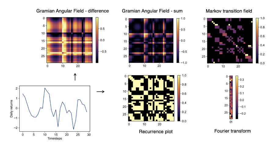
Figure 5: 2D timeseries
Following Wang & Oates [4], we can represent our time-series as a 2D space using the Gramian sum angular field (GSAF), Gramian difference angular field (GDAF), and the Markov transition field (MTF) transforms. We can also represent a time-series as a recurrence plot (RP), or by its Fourier transform (with real and imaginary components stacked so as to form a narrow image). These transforms are shown in Figure 5, implemented after Faouzi & Janati [5] for a historical returns time-series. Each transform shows its own idiosyncrasies and tends to highlight specific behaviours and features. Considering application to synthetic data in Figure 6, we take a closer look at how varying the frequency of a simple sine wave affects its GSAF transform.
Figure 6: The GSAF transform of a sine wave
With such transforms at our disposal, we can convert the time-series of equity prices, individual company fundamentals, and macroeconomic indicators (like US GDP, $ to £ exchange rate, etc) into 2D representations. This lets us consider slices of a market as a stack of images. For example, over the same 60-day period we could have images corresponding to each of asset daily returns, daily highest price, daily lowest price, with each pixel representing a single day. This makes up a data stack akin to the red, green, blue layers of a coloured digital image. Recent research from Zhang et al [6] applies a similar approach directly to a limit order book in order to aid predictions of financial instruments.
Machine learning is about transforming complicated data into useful representations. CV techniques are very powerful in learning the extremely complex interactions between pixels in an image of a cat, to the degree that they can distinguish it from those of a dog. This is achieved by learning to look for (and distinguish between) the abstract features of 'dog ear' vs 'cat ear'. By exploiting the translational symmetries shared between time-series and natural images, CNNs are able to efficiently identify these complex interactions.
We have the choice to use such techniques in either a supervised or unsupervised learning paradigm. In the former, one may train a classification model to take such images as inputs, and predict a future price movement, similarly to classifying an image as containing a cat or a dog. In this setting we would provide a corresponding label to each image (or set of images), representing examples of the mapping from image(s) to label we wish to learn. In an unsupervised setting, we provide data but no labels. An auto-encoder model compresses the information stored in, for example, an image down to a handful of representative (hidden) features, which it then uses to reconstruct the input as accurately as possible[3]. Presented in Figure 7 is an example of a CNN auto-encoder trained to reconstruct GSAF-transformed features of a time-series. The input can be reconstructed well, meaning the low-dimensional representations we access through this model contain the same information as the original data.
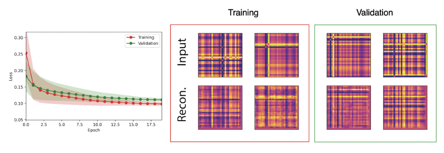
Figure 7: GSAF reconstructions of a financial time-series dataset
Learning to find the most important parts of the dataset with unsupervised learning increases the efficiency with which we can handle data, reducing compute cost and permitting more algorithmic complexity. Convolutional architectures do this extremely well for images, and other data with translational symmetry. Identifying key features of a time-series with unsupervised learning remains an important research focus for us.
At Arabesque AI, we aim to forecast stock market movements using a wide range of models, but finding useful features of very noisy data remains a key challenge. We research and develop the powerful technology discussed in this post towards our core objective: accurately forecasting stock market movements with cutting edge machine learning.
[1] Note that this operation, performed in CNNs, is actually a cross-correlation rather than a convolution. The misnomer is due to the fact that a convolution operation flips the kernel before calculating the dot product, such that a copy of the filter is obtained from a convolution with a unit 'impulse'. As CNNs are already a complex system, and we do not care about this specific property we drop the filter flipping, making the operation technically a cross-correlation. In the case of Figure 2, the symmetric filters mean that the convolution and cross-correlation operations are identical, but in CNNs the learned filters need not be symmetric.
[2] Note that the concept of 'scanning' is what is mathematically happening in this operation. This would be an inefficient algorithmic implementation.
[3] This is similar to the function of principal component analysis (PCA), widely used in quantitative finance to remove the market factor from a portfolio's performance, but an auto-encoder can identify complex non-linear interactions that PCA does not see.
References
-
Fei-Fei, L. Deng, J. Li, K. (2009). "ImageNet: Constructing a large-scale image database." Journal of Vision, vol. 9 http://journalofvision.org/9/8/1037/, doi:10.1167/9.8.1037
-
Krizhevsky, A. Sutskever I., Hinton, G.E. (2012). "ImageNet classification with deep neural networks," Communications of the ACM, vol 60 (6), pp 84–90, doi:10.1145/3065386
-
R. W. Fleming and K. R. Storrs. (2019). "Learning to see stuff," Current Opinion in Behavioural Sciences, vol. 30, pp. 100–108.
-
Wang, Z. and Oates T. (2015). "Imaging time-series to improve classification and imputation," International Joint Conference on Artificial Intelligence, pp. 3939 – 3945.
-
Faouzi, J. and Janati, H. (2020). "pyts: A python package for time series classification," Journal of Machine Learning Research, 21(46): pp. 1−6.
-
Zhang, Z. Zohren, S., Roberts, S. (2019) "DeepLOB: Deep convolutional neural networks for limit order books," IEEE Transactions on Signal Processing, 67 (11): pp. 3001 – 3012.